Use of Python in the biological environment- Prey Predators Equation (Lotka–Volterra model)

23 May 2022 - Ashma Subedi

Ashma Subedi recently completed her Masters in Environment Science from Kathmandu University. She loves solving environment problems using data science and machine learning, especially time series analysis.

The relation and interactions between predators and their prey are important factors when it comes to conservation and ecosystem stability. In an ecosystem, the predator/prey relationship provides enough stability for an essentially unlimited number of species to coexist. Predators, for example, enhance predation and reduce the number of prey when the number of prey is high. Ecosystems are more stable and can support a greater number of species as a result of these predator/prey relationships.

Let’s see an example of prey and predator of Chitwan National Park. Every day, deer or wild boar must run faster than the fastest tiger or get unnoticeable around the tiger, if not it will be killed. Likewise, the tiger knows it must outrun the slowest deer or it will starve to death.

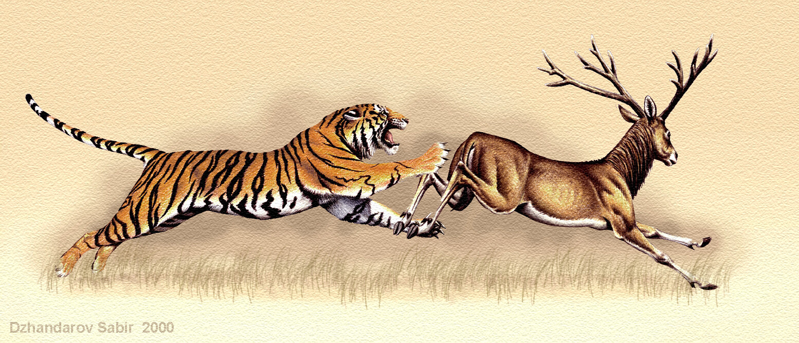
Source: https://suleimansultan.artstation.com/projects/zOXLl6

So what are the laws that govern the dynamics of these prey and predator’s complicated systems and how do these species interact? To answer these questions ordinary differential equation (ODE) model can be used, which consists of two animal species, one that acts as a predator species and the other as its prey: the prey-predator model, also known as Lotka–Volterra equations.

To understand the interesting relationship between prey and predators and to get the answer to the above-mentioned questions, I took the initiative to work on a biological model “Dynamics of Biological Systems in which Tiger and Deer interact” using Python.

This blog will highlight some of the Python skills (such as the use of matplotlib module and its application to plot trajectories, directions fields, etc.) which I have acquired from Data Fellowship, Code for Nepal. The main objective of this blog is to describe the dynamics of ecological systems in which two species interact.

The Lotka–Volterra Model

The populations change through time according to the pair of equations:

du/dt =a*u-b*u*v(dv/dt)=-c*v +d*b*u*v

with the following notations:

u: number of preys (for example, deer)
v: number of predators (for example, tigers)
a, b, c, d are constant parameters defining the behavior of the population:
a is the natural growth rate of deer when there’s no tiger
b is the natural death rate of deer, due to predation
c is the natural death rate of tigers when there’s no deer
d is the factor describing how many caught deer let’s create a new tiger

Here a, b, c, and d are some given constants.

Firstly, all the necessary libraries were imported and the constant parameters were defined (example: a= 1, b=0.1, c=1.5, d=0.75).

Population equilibrium and stability of fixed points

When neither of the population levels changes, i.e. when both of the derivatives are equal to 0, the model is said to be in population equilibrium. This results in two fixed points, and the stability of the fixed point at the origin can be determined using partial derivatives and linearization.

A saddle point on the surface of a function’s graph, where the slopes (derivatives) in orthogonal directions are all zero, is the function’s origin (a critical point). This point is important because it shows the stability of the function. If the system is stable, then the extinction of both species would be very unlikely. However, since the origin point is unstable, it is hard to predict the extinction of both species. If the predators are intentionally destroyed, then the prey population would only grow, and the predators would die of starvation. This scenario would only occur if the populations of both the predators and the prey are destroyed. Prey and predator populations can go infinitesimally near to extinction and still recover.

Integrating the ordinary differential equations using scipy.integrate

This module has an odeint function for integrating ODEs that can be used by importing a library (from scipy import integrate). After the integration, the following figure is obtained which shows the possible solutions to the Lotka-Volterra equations.

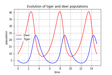
The example exemplifies the model’s key qualitative behavior and its ever-changing character. These variations are unavoidable in a real-world system. When predators are few, the prey population has a chance to expand since predators may catch fewer animals than new prey are born. However, if the prey population is large enough, many predators will be content enough to have progeny.

The rising predator population will consume more prey until it reaches a point where consumption exceeds prey reproduction. After that, the prey population will begin to dwindle. Because of the decreased supply of food, the predator population will soon follow, resulting in mass starvation. The ecology will be in a position where there are few preys and few predators, allowing the prey population to rise once more, and history will repeat itself.

Different starting points between the extinction of both species were plotted in a phase plane, and Matplotlib’s colormap was used to define colors for the trajectories.

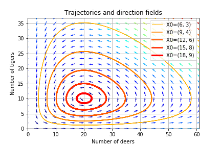
Figure: Phase-space plot for the predator and prey

Changing the tiger or deer population can have unexpected consequences. If tigers are introduced to reduce the number of deers, this may result in an increase of deers, in the long run, depending on the timing of the intervention.

In conclusion, ecologists and biologists can use this model to predict what will happen when two species compete for the same resources. Furthermore, predators influence the dynamics of their prey in ways that cascade across ecosystems, altering processes such as productivity, biodiversity, nutrient cycles, disease dynamics, carbon storage, etc. However, this model requires certain assumptions (as made here also) that may or may not be true in the natural world. Some assumptions include: the prey population always has enough food, the population’s rate of change is proportional to its size, predators have an insatiable desire, etc.

Because of Code For Nepal’s Data Fellowship program in partnership with DataCamp Donates, I was able to take the initiative to learn more about the Lotka–Volterra model and its applications. I am grateful to Code for Nepal for providing me with the opportunity to study advanced Python.